Example 3: Phase Entropy w/ Pioncare Plot

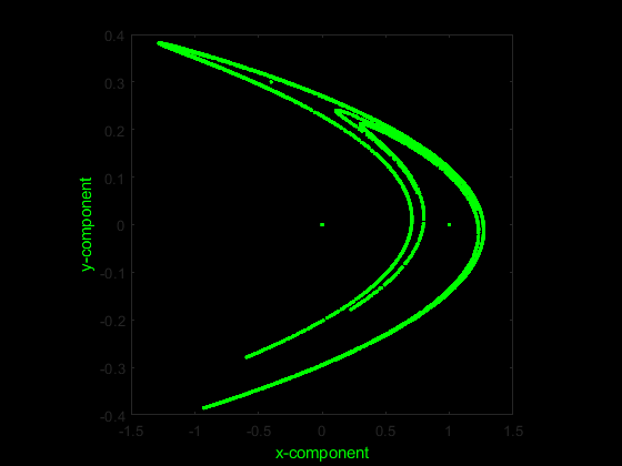
Import the x and y components of the Henon system of equations.

Data = ExampleData('henon');

figure('Color', 'k')
plot(Data(:,1), Data(:,2), 'g.')
xlabel('x-component','color','g'),
ylabel('y-component','color','g')
set(gca,'color','k'), axis square

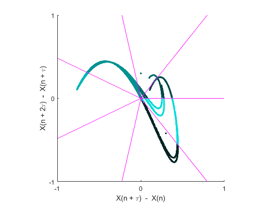
https://github.com/MattWillFlood/EntropyHub/blob/main/Graphics/henon.png?raw=true

Calculate the phase entropy of the y-component in bits (logarithm base 2) without normalization using 7 angular partitions and return the second-order difference plot.

Y = Data(:,2);
Phas = PhasEn(Y, 'K', 7, 'Norm', false, 'Logx', 2, 'Plotx', true)

>>> Phas = 2.0193

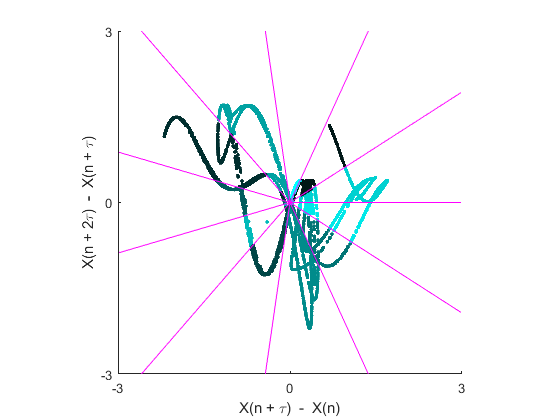
https://github.com/MattWillFlood/EntropyHub/blob/main/Graphics/phasex1.png?raw=true

Calculate the phase entropy of the x-component using 11 angular partitions, a time delay of 2, and return the second-order difference plot.

X = Data(:,1);
Phas = PhasEn(X, 'K', 11, 'tau', 2, 'Plotx', true)

>>> Phas = 0.8395