Example 9: Hierarchical Multiscale corrected Cross-[Conditional] Entropy

Import the x and y components of the Henon system of equations and create a multiscale entropy object with the following parameters:

EnType = XCondEn(), embedding dimension = 2, time delay = 2, number of symbols = 12, logarithm base = 2, normalization = true

from matplotlib.pyplot import figure, plot, axis

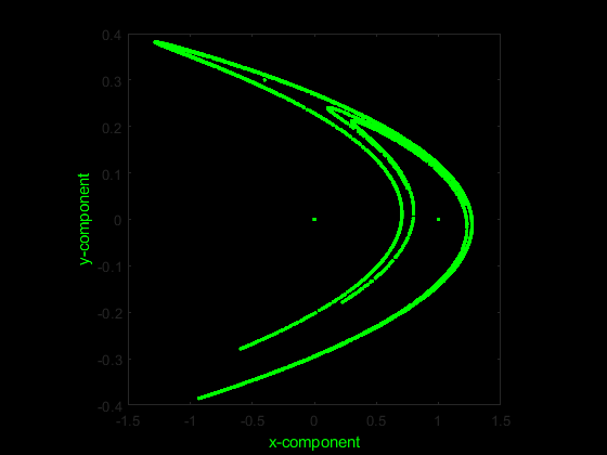
Data = EH.ExampleData('henon');

fig = figure(facecolor='k')
plot(Data[:,0], Data[:,1], 'g.')
axis('off')

Mobj = EH.MSobject('XCondEn', m = 2, tau = 2, c = 12, Logx = 2, Norm = True)

Mobj.Func
>>> <function EntropyHub._XCondEn.XCondEn(Sig, m=2, tau=1, c=6, Logx=2.71828, Norm=False)>

Mobj.Kwargs
>>> {'m': 2, 'tau': 2, 'c': 12, 'Logx': 2, 'Norm': True}

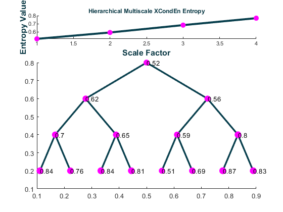
Calculate the hierarchical multiscale corrected cross-conditional entropy over 4 temporal scales and return the average cross-entropy at each scale (Sn), the complexity index (Ci), and a plot of the multiscale entropy curve and the hierarchical tree with the cross-entropy value at each node.

MSx, Sn, Ci = EH.hXMSEn(Data[:,0], Data[:,1], Mobj, Scales = 4, Plotx = True)

>>> WARNING: Only first 4096 samples were used in hierarchical decomposition.
The last 404 samples of each data sequence were ignored.
. . . . . . . . . . . . . . . . . .

>>> MSx =
    array([0.5159, 0.6245, 0.5634, 0.7022, 0.6533, 0.5853, 0.7956, 0.8447,
           0.7605, 0.8415,0.8115, 0.5128, 0.6862, 0.8679, 0.8287])
    Sn =
    array([0.5159, 0.5940, 0.6841, 0.7692])
    Ci =
    2.5632