Example 12: [Generalized] Refined-composite Multivariate Multiscale Fuzzy Entropy

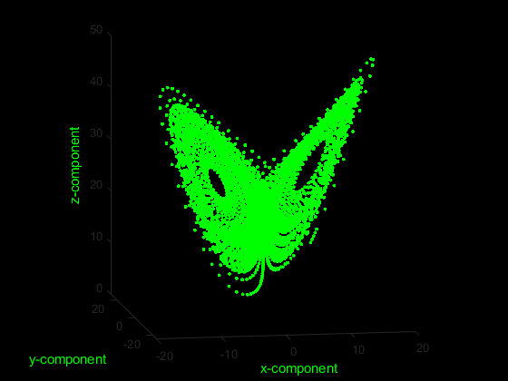
Import the x, y, and z components of the Lorenz system of equations.

Data = EH.ExampleData('lorenz')

from matplotlib.pyplot import fig, scatter, axis

fig = figure(facecolor='k')
ax = fig.add_subplot(111, projection='3d')
ax.set_facecolor('k')
ax.scatter(Data[:,0], Data[:,1], Data[:,2], c='g')
ax.axis('off')

Create a multiscale entropy object with the following parameters: EnType = MvFuzzEn(), fuzzy membership function = ‘constgaussian’, fuzzy function parameter = 1.75, normalized data to unit variance = true.

Mobj = EH.MSobject('MvFuzzEn', Fx = 'constgaussian', r = 1.75, Norm = True)

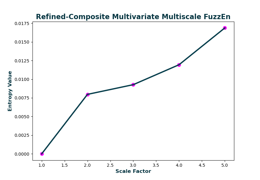
Calculate the generalized refined-composite multivariate multiscale fuzzy entropy over 5 scales and plotting the output.

Hint

When the multivariate entropy method is multivariate fuzzy entropy (MvFuzzEn), cMvMSEn by default employs a generalized graining procedure with the standard deviation (not the variance like in MvMSEn). This follows the method presented in [1].

[1] Azami, Fernández and Escudero. ” Refined multiscale fuzzy entropy based on standard deviation for biomedical signal analysis ” Medical & biological engineering & computing 55 (2017): 2037-2052

Caution

As with conventional generalized multiscale entropy, the multiscale entropy value for the first scale will always == 0, as the variance or standard deviation of a singular value is 0!

MSx, CI = EH.cMvMSEn(Data, Mobj, Scales = 5, Refined = True, Plotx = True)

>>> MSx =
    0,  0.00796833,  0.00926765,  0.01193731,  0.01686631

>>> RDE =
    0.04603960